
Data Partitioning
Data Partitioning is critical to Spark performance, specially for large volumes of datasets that are to be joined with another dataset. Spark assigns one task for each partition and each worker thread can only process one task at a time. With too few partitions, Spark won’t be able to utilize all the cores available in the cluster resulting in data-skew problem. On the other hand – too many partitions introduce overhead for Spark to manage too many tasks. It’s very important to partition data appropriately on the columns that are in the filter clause of the query or columns on which data-fra mes are joined.
What is a Partition in Spark?
A logical atomic chunk of data. In Spark, partitions are distributed among nodes in logical chunks. Partitions are basic unit of parallelism in Spark. Shuffling refers to movement of data amongst these partitions spanning across the nodes in the cluster. Spark can run the same task concurrently for every partition of the dataset – thereby allowing massively parallelized processing in a distributed environment.
Why is Shuffling an issue?
Shuffling inherently involves marshalling and unmarshalling which is a pre-requisite for data storage and transmission across the network. Typically, when data must be moved between different parts of a physical or logical storage, it needs to be serialized (marshalled) and deserialized (unmarshalled), which means data must be transformed from the memory representation to a format suitable for transmission and then back to the memory representation for the storage after the transmission.
Cores and Partitions Relationship
Partitions should be a multiple of the total number of cores in the cluster. E.g. If your cluster has 100 cores, you should have at least 100 partitions to allow for 1:1 ratio of Parallelism in Spark. In practice, the number of partitions should be 3-5 x more than the number of cores. If you have 100 cores and 500 partitions of the dataset, the parallelism ratio would be 1:5, that means 100 cores (a task is running on a core, which is a Java Virtual Machine). It is important to keep in mind that each executor node typically has 2 to 4 vCores. More powerful executor machines may have 8 vCores. Each executor is a physical EC2 node with 16 GB, 32 GB or 64 GB RAM depending on the hardware appliance. A 32 GB executor node with 4 vCores means each vCore has 8 GB of RAM, running its own JVM. You should always set aside 20% of the vCore RAM for the heap size, the remaining 80% is the actual processing power of the vCore, logically available to run a task in parallel.
What is Parallelism?
Parallelism is a distributed computing paradigm that refers to each task independently and concurrently processing a logical chunk of data.
What is a task? A Stage? A Job?
A task is a unit of work that is sent to the executor by Spark’s Driver program. Each Stage comprises of tasks, one task per partition.
Lazy Evaluation – In Spark, a task is not executed until an action is performed. collect(), take() and show() are examples of action.
When code is submitted to Spark, the Driver program analyzes the code and breaks it into Jobs. Each Job comprising of 1 or more Stage, each Stage comprising of 1 or more tasks – depending on the number of vCores in the Cluster.
RDD
Resilient Distributed Dataset, a resilient dataset in Spark that is distributed across nodes in the cluster. RDDs get partitioned automatically without programmer’s intervention. However, most of the time while dealing with massive analytical ETL or realtime workloads, you would like to adjust the size and number of partitions or the partitioning scheme to the needs of your analytics use-case.
Code Examples:
Partition dataset with parallelize() API
Using Jupyter Notebook with Spark 2.4 and Python 3.7 to run as PySpark on localhost with “local[4]“, meaning a 4 vCores cluster.

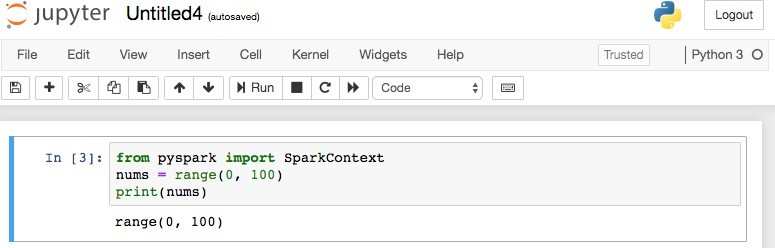
Here, we import SparkContext from pyspark. SparkContext is the entry point, the Driver program per say, which is responsible for distributing the datasets and tasks across the cluster. The dataset is a Python array of comma separated numbers from 0 to 99.
In Jupyter Notebook, SparkContext is already initialized and available as sc. If you are not using Jupyter Notebook, then initialize the SparkContext like this:
with SparkContext(“local[4]”) as sc:
Spark uses different partitioning schemes for various types of resilient distributed datasets (RDD) and operations. Below are the code snippets of these partitioning schemes.
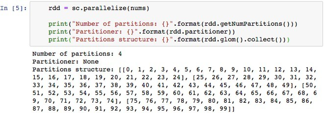
parallelize(nums) – Spark evenly distributes dataset across vCores. We are parallelizing python array containing 100 comma separated values into an RDD with no partitioning scheme.
glom() – API exposes the structure of created partitions. It returns an RDD created by coalescing all elements within each partition into a list. Each RDD also possesses information about partitioning schema. You will observe, the dataset of 100 records – nums – is split into 4 equal partitions, each containing 25 records, as the cluster has 4 vCores available. This means we allowed the Spark Driver program to use four local vCores, each vCore is capable of running the task in parallel. This is the ideal situation for parallelism, where each vCore will be able to operate on one partition.
partitioner – inspects partitioner information used to partition the RDD.
In general, smaller, more numerous partitions allow work to be distributed among more workers (Stage comprising of more tasks).
Larger and fewer partitions allow work to be done in larger chunks, reducing shuffle between the nodes. Spark can only run 1 concurrent task for every partition of the RDD, up to the number of cores in your cluster. So, if you have a cluster with 100 cores, you want your RDDs to at least have 100 partitions, possibly even 3-4 x the number of cores.

Here, we increase the number of partitions from 4 to 15. Each partition now has 6 or 7 records. Now 4 tasks can run in parallel on smaller partitions and possibly process faster. As soon as the task completes processing a partition, it can start on the next un-processed partition.
Custom partitions using partitionBy()
Allows applying custom partitioning logic over the dataset.

partitionBy() requires dataset to be in key/value (pair) objects referred to as tuples.
map(lambda num: (num, num)) – lambda function transforms the dataset’s each element into a key,value pair commonly referred to as tuple.
In this example, since the nums dataset already contained unique values, each value is also now a key to itself. Now the PairRDD contains 100 objects of k,v pair such that it can be unpacked as k, v = kv
partitionBy(2) – Split the dataset into 2 chunks, using default hash partitioner. Elements are now distributed into 2 partitions.
To determine which records go to what partition, Spark uses partition function. The partition to which a particular record is added depends on the partition_key and the number of partitions. In the example above, all even numbered keys were added to the same partition, and the odd numbered keys were added to another partition.
partition = partitionFunc(key) % num_partitions – See the example below.

The code above uses hash_function % number of partitions to determine the partition to assign the records to. Since there are only 2 partitions, partition 0 and partition 1, records are assigned to either one based on the hash of the key modulus 2.
Custom Partitioner using hash function
Given a tuple key, function returns an integer – that integer % the number of partitions determines the partition to assign the records to.
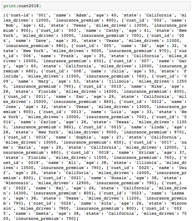
With a custom partitioner, we can see what partition each state is assigned to, ensuring that records of one state are on the same node. This strategy can greatly reduce network traffic, avoiding shuffle of records belonging to the same state. In the absence of this customized hash partitioning, records of one state will be scattered all over the cluster on different nodes/partitions, causing latency during shuffle. Before performing any joins or aggregation function in Spark, it is extremely important to ensure that records that have a common key are colocated.Consider the dataset below with 25 records from 5 states in JSON format.
cust2018 = [
{‘cust_id’ : ‘001’ , ‘name’: ‘Adam’, ‘age’: 40, ‘state’: ‘California’, ‘miles_driven’: 12000, ‘insurance_premium’: 800},
{‘cust_id’ : ‘002’ , ‘name’: ‘Bob’, ‘age’: 42, ‘state’: ‘Texas’, ‘miles_driven’: 13000, ‘insurance_premium’: 900},
{‘cust_id’ : ‘003’ , ‘name’: ‘Cathy’, ‘age’: 41, ‘state’: ‘New York’, ‘miles_driven’: 10000, ‘insurance_premium’: 700},
{‘cust_id’ : ‘004’ , ‘name’: ‘Dave’, ‘age’: 30, ‘state’: ‘Texas’, ‘miles_driven’: 11000, ‘insurance_premium’: 980},
{‘cust_id’ : ‘005’ , ‘name’: ‘Ed’, ‘age’: 32, ‘state’: ‘New York’, ‘miles_driven’: 9000, ‘insurance_premium’: 970},
{‘cust_id’ : ‘006’ , ‘name’: ‘Frank’, ‘age’: 35, ‘state’: ‘California’, ‘miles_driven’: 10000, ‘insurance_premium’: 650},
{‘cust_id’ : ‘007’ , ‘name’: ‘Gary’, ‘age’: 60, ‘state’: ‘California’, ‘miles_driven’: 12000, ‘insurance_premium’: 680},
{‘cust_id’ : ‘008’ , ‘name’: ‘Julia’, ‘age’: 55, ‘state’: ‘Florida’, ‘miles_driven’: 11500, ‘insurance_premium’: 760},
{‘cust_id’ : ‘009’ , ‘name’: ‘Mary’, ‘age’: 53, ‘state’: ‘Illinois’, ‘miles_driven’: 13500, ‘insurance_premium’: 790}
{‘cust_id’ : ‘0010’ , ‘name’: ‘Mike’, ‘age’: 28, ‘state’: ‘Florida’, ‘miles_driven’: 14000, ‘insurance_premium’: 800},
{‘cust_id’ : ‘0011’ , ‘name’: ‘Zac’, ‘age’: 29, ‘state’: ‘California’, ‘miles_driven’: 15000, ‘insurance_premium’: 860},
{‘cust_id’ : ‘0012’ , ‘name’: ‘Jose’, ‘age’: 32, ‘state’: ‘Texas’, ‘miles_driven’: 13000, ‘insurance_premium’: 900},
{‘cust_id’ : ‘0013’ , ‘name’: ‘Luis’, ‘age’: 33, ‘state’: ‘New York’, ‘miles_driven’: 10000, ‘insurance_premium’: 700},
{‘cust_id’ : ‘0014’ , ‘name’: ‘Carlos’, ‘age’: 26, ‘state’: ‘Texas’, ‘miles_driven’: 11000, ‘insurance_premium’: 980},
{‘cust_id’ : ‘0015’ , ‘name’: ‘Linda’, ‘age’: 28, ‘state’: ‘New York’, ‘miles_driven’: 9000, ‘insurance_premium’: 970},
{‘cust_id’ : ‘0016’ , ‘name’: ‘Sophia’, ‘age’: 27, ‘state’: ‘California’, ‘miles_driven’: 10000, ‘insurance_premium’: 650},
{‘cust_id’ : ‘0017’ , ‘name’: ‘Maria’, ‘age’: 29, ‘state’: ‘California’, ‘miles_driven’: 12000, ‘insurance_premium’: 680},
{‘cust_id’ : ‘0018’ , ‘name’: ‘Sriram’, ‘age’: 37, ‘state’: ‘Florida’, ‘miles_driven’: 11500, ‘insurance_premium’: 760},
{‘cust_id’ : ‘0019’ , ‘name’: ‘Ali’, ‘age’: 38, ‘state’: ‘Illinois’, ‘miles_driven’: 13500, ‘insurance_premium’: 790},
{‘cust_id’ : ‘0020’ , ‘name’: ‘Usuf’, ‘age’: 26, ‘state’: ‘Califoria’, ‘miles_driven’: 14000, ‘insurance_premium’: 800}
{‘cust_id’ : ‘0021’ , ‘name’: ‘Husain’, ‘age’: 38, ‘state’: ‘Wisconsin’, ‘miles_driven’: 12900, ‘insurance_premium’: 790},
{‘cust_id’ : ‘0022’ , ‘name’: ‘Raj’, ‘age’: 26, ‘state’: ‘California’, ‘miles_driven’: 14300, ‘insurance_premium’: 800},
{‘cust_id’ : ‘0023’ , ‘name’: ‘Laxman’, ‘age’: 38, ‘state’: ‘Texas’, ‘miles_driven’: 11200, ‘insurance_premium’: 790},
{‘cust_id’ : ‘0024’ , ‘name’: ‘Sita’, ‘age’: 26, ‘state’: ‘Wisconsin’, ‘miles_driven’: 7800, ‘insurance_premium’: 800},
{‘cust_id’ : ‘0025’ , ‘name’: ‘Geeta’, ‘age’: 38, ‘state’: ‘California’, ‘miles_driven’: 7500, ‘insurance_premium’: 790}
]
Now, parallelize and distribute cust2018 dataset such that records of one state are on the same partition, using the custom state_partitioner.
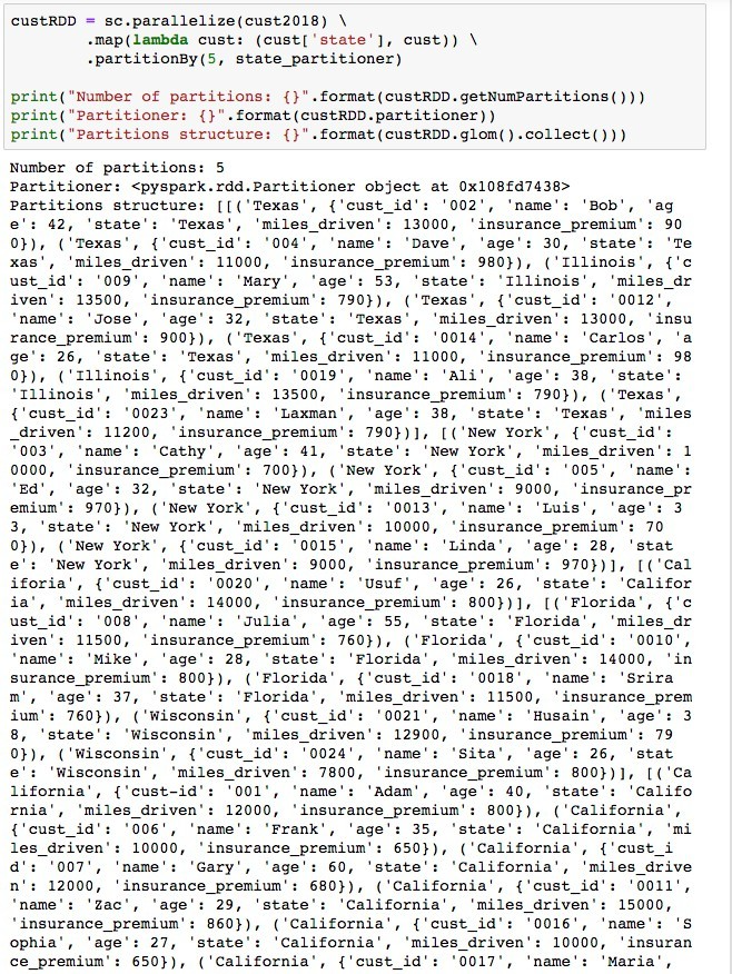

Now that all records from the state are in the same partition, it is much easier for a task to work directly on those partitions without worrying about shuffling.
mapPartitions()
Converts each partition of the source dataset into multiple elements of the result (possibly none). mapPatitions() allows heavyweight initialization to be done once for many elements in each partition, instead of running map() for each element in the dataset.
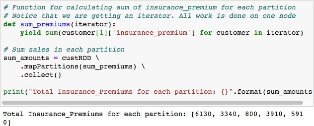
As an example, to calculate the sum of insurance premiums in each state, mapPartitions() API can be efficiently used without any shuffling of data between partitions.
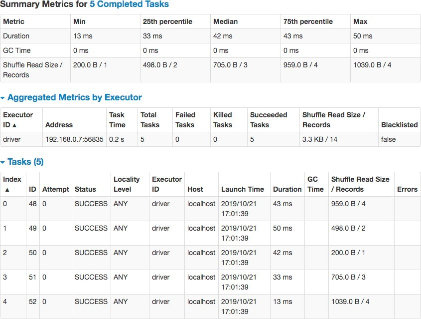
If map() was used instead of mapPartitions() in the code snippet above, map() function will be called 25 times, once for every row in the dataset. mapPartitions() is much faster than map() because, it operates on many rows in the same partition, thus the function is invoked only once per partition for heavyweight initialization. You can achieve 300x performance increase using mapPartitions() in group-by and aggregate functions over map(). In the web-ui at port 4040, notice minimal shuffle read in mapPartitions() operation and no garbage collection. There are 5 tasks, because we partitioned the custRDD by 5 on state key.

DataFrames and Datasets
Unlike RDD, DataFrames organize data into named columns, like a table in a relational database. Organizing structured or semi-structured data into named columns allows Spark to infer the schema of the DataFrame. Like RDD, DataFrame is also immutable, lazily evaluated and distributed collection of data. Dataset – available only in Scala and Java – are an extension of DataFrame API which provides type-safe, object-oriented programming interface. Dataset takes advantage of Spark’s Catalyst Optimizer by exposing expressions and data fields to a query planner. Use Datasets wherever possible. In case of Python, use DataFrames API instead of RDD. It is very easy to create custom partitioners with DataFrames and Datasets.
repartition() – custom partitioner in DataFrame
Code below shows how to use repartition() on a DataFrame to control parallelism in Spark.
# You can also repartition with numPartitions and column_name as below.
df 2 = df.repartition(5,”state”)
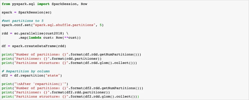
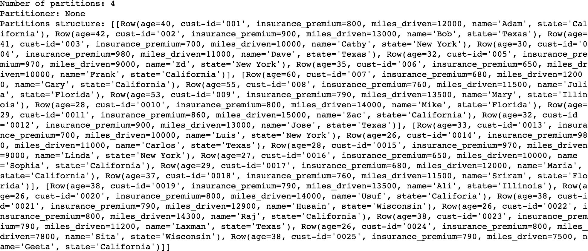
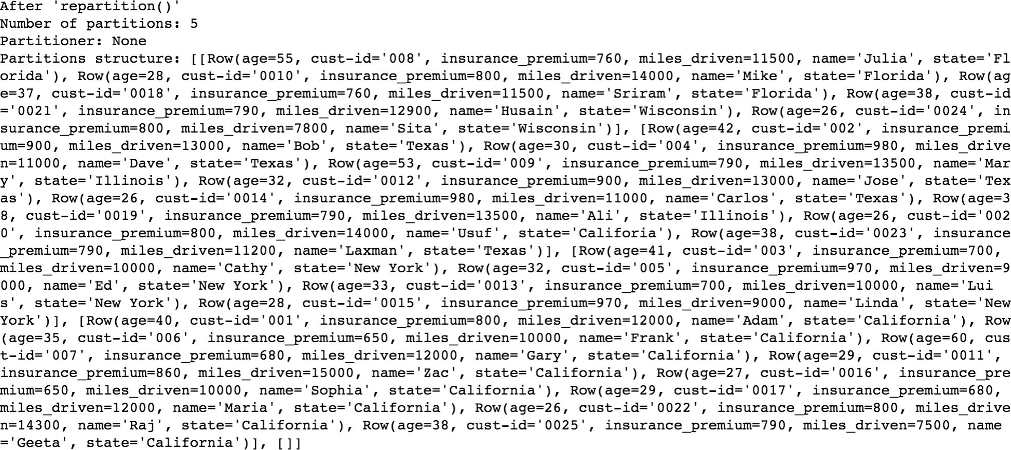
When you first create the DataFrame, it partitions the dataset in to 4 partitions as the available vCores are 4 in the cluster.
When the repartition() API is invoked with column name, it repartitions the dataset into 5 partitions – as per the parameter set in spark.sql. shuffle.partitions. It is much simpler to repartition the DataFrame with column names and also control the number of partitions to create for the HashPartitioner. Default value for spark.sql.shuffle.partitions is 200, which means when a full shuffle forces a new Stage, there will be 200 partitions, and thereby 200 tasks in that Stage. When you are dealing with millions or billions of records and GB or PB scale dataset, partitioning the dataset on appropriate column(s) and the number of partitions is critically important for optimal performance.
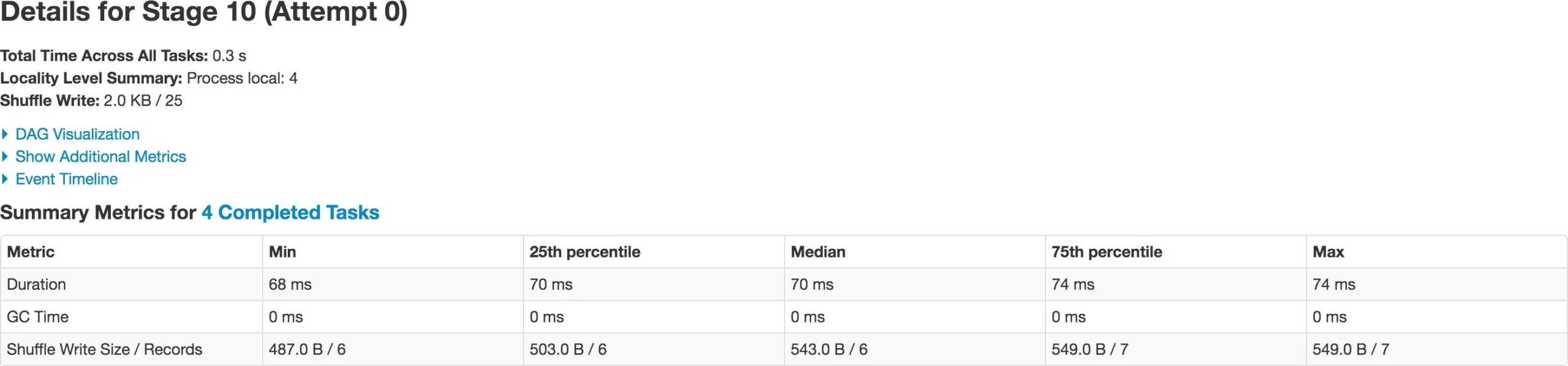
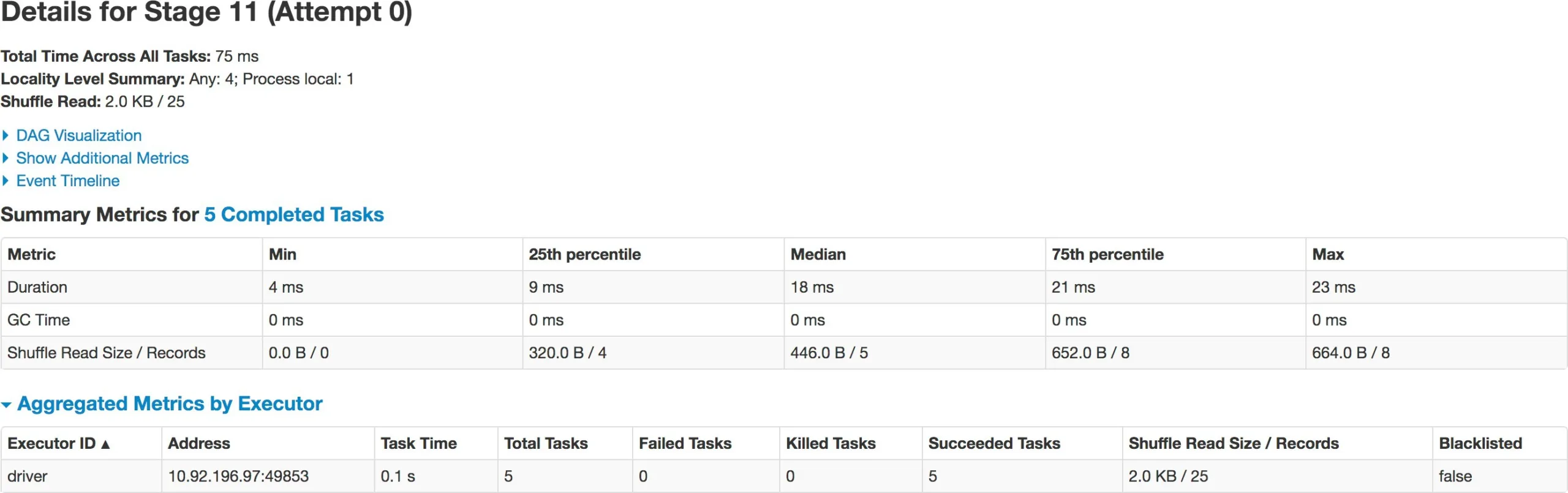
repartition() performs full shuffle, as data must be shuffled across nodes. Spark handles full shuffle in a new Stage – comprising of tasks equal to the number of partitions. When you first create the DataFrame there are 4 partitions of the dataset. As soon as you repartition the DataFrame to 5 – it forces a new Stage – now comprising of 5 tasks. This way, you can increase or decrease parallelism in Spark by controlling the number of partitions of your dataset. Also note, repartition() took half the time (37 ms) of original DataFrame creation (79 ms).

Benefit of partitioning in shuffle operations
All operations performing data shuffle by key inherently benefit from partitioning. Examples are groupByKey(), groupWith(), cogroup(), reduceByKey(), combineByKey(), join(), leftOuterJoin(), rightOuterJoin(), lookup(). These operations cannot modify the key of the element in the record, so they can retain the parent DataFrame’s Partitioner.
Use mapValues() instead of map()
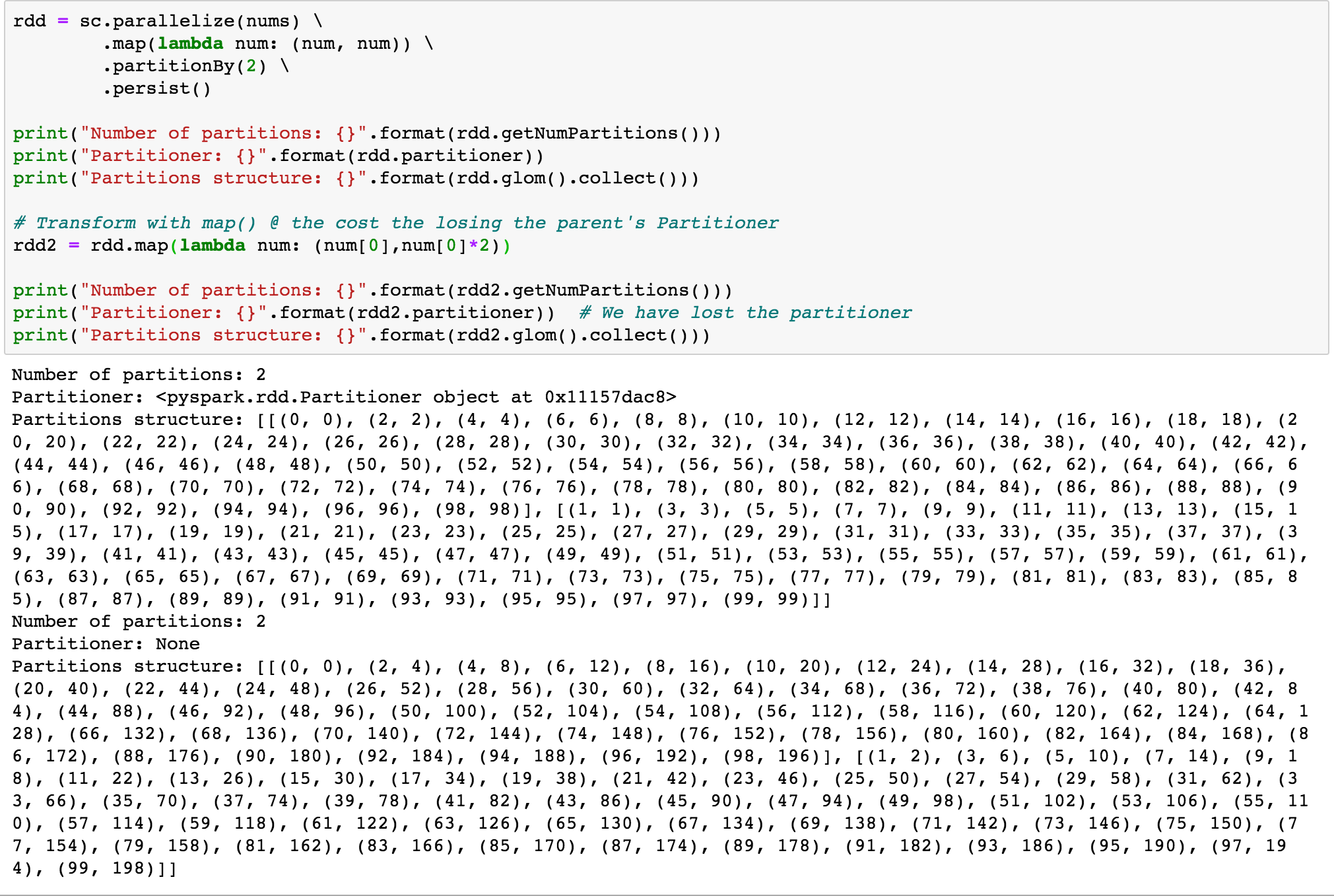
map() transformation can possibly modify the key of each element in the record as shown in the code above, Spark cannot guarantee to produce known partitioning, so map() operation cannot retain the parent DataFrame or RDD’s Partitioner.
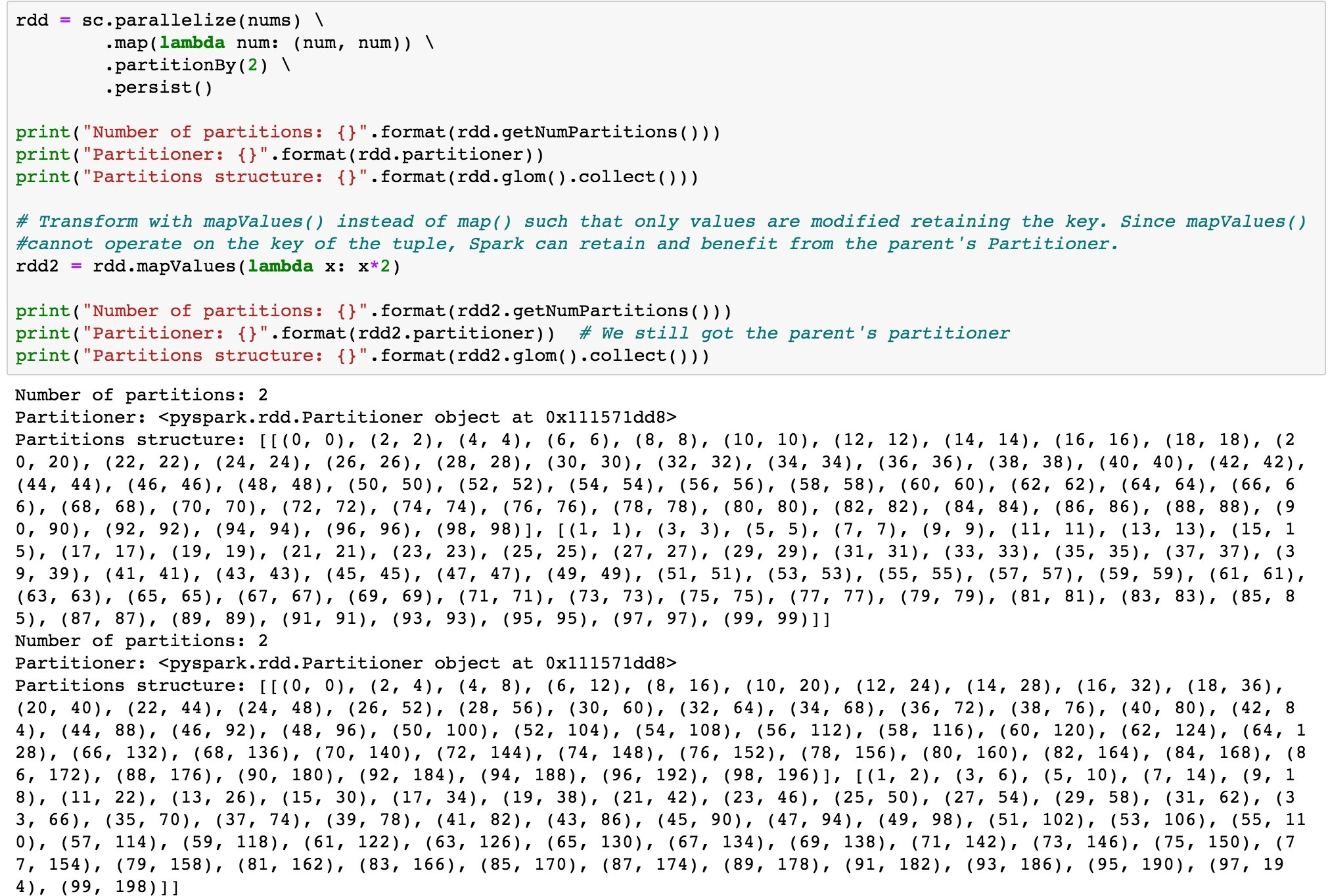
mapValues(), flatMapValues() and filter() operations guarantee that each tuple’s key remains the same and may benefit from the parent DataFrame’s Partitioner.
The Code below shows transformation of the parent RDD using map() which forgoes the parent’s Partitioner and the same transformation using mapValues() which retains the parent RDD’s partitioner.
Data Format
RDD – Can process structured and un-structured data, but cannot infer schema of ingested data. Developer needs to specify the schema.
DataFrame – Can process structure and semi-structured data. Organizes data into named columns. Allows Spark to infer schema.
Optimization
RDD – No built-in optimization engine is available on RDDs in Spark. RDDs cannot take advantage of Spark’s Catalyst Optimizer.
DataFrame – Built-in optimization using Catalyst Optimizer. DataFrames use catalyst transformation framework in 4 phases: 1) analyzing a logical plan to resolve references, 2) Logical plan optimization, 3) physical plan, 4) code generation
Aggregation
RDD – Slower to perform simple grouping and aggregation operations on RDD.
DataFrame – Easy to use and faster on large data sets.
Coalesce()
Decreases the number of partitions minimizing shuffles.
Code to Follow:
Data Skew
If some partitions have a lot more records than the other partition, the task will take longer to process the partition with more data, possibly leading to data skew that results in sub-optimal use of the resources. It is important to set a limit for the number of records in every partition such that data is evenly distributed among partitions to avoid data skew. Data Skew is a data problem and needs to be resolved at the data level. The root cause of data skew is uneven distribution of the underlying data on heavily skewed keys. During join and group-by key operations, null values in join keys or group-by keys also result into data skew.
Identifying Data Skew
You observe all but few tasks in a Stage finishing within a reasonable time-frame. Often only 1 task takes forever to finish or never finishes.
Resolve Data Skew
If join operation is done on a skewed dataset, a quick trick to prevent data skew is to increase the ‘spark.sql.autoBroadcastJoinThreshold’ value, so the smaller table on the right side of the join is broadcast to all the nodes in the cluster. Before enabling autoBroadcastJoinThreshold, ensure there is sufficient driver and executor memory.
If there are too many null values in the dataset, pre-process those null values with some random ids, and handle those random ids in the application code, after the join.
Use salting on the join key to redistribute data in an even manner, so that that the task processing on that partition completes in a reasonable time-frame.
Salting
Is a technique where random values are added on join key of the left table. On the right table, rows are replicated to match the random keys, in such a way that if leftTable.key1 == rightTable.key1, then leftTable.key1_<salt> == leftTable.key1_<salt>.
Code Example: To be added
raw-code: Below is the raw code from PySpark’s ipython notebook.
from pyspark import SparkContext nums = range(0, 100) print(nums)
rdd = sc.parallelize(nums)
print(“Number of partitions: {}”.format(rdd.getNumPartitions())) print(“Partitioner: {}”.format(rdd.partitioner)) print(“Partitions structure: {}”.format(rdd.glom().collect()))
rdd = sc.parallelize(nums, 15)
print(“Number of partitions: {}”.format(rdd.getNumPartitions())) print(“Partitioner: {}”.format(rdd.partitioner)) print(“Partitions structure: {}”.format(rdd.glom().collect()))
rdd = sc.parallelize(nums) \
.map(lambda num: (num, num)) \
.partitionBy(2) \
.persist()
print(“Number of partitions: {}”.format(rdd.getNumPartitions())) print(“Partitioner: {}”.format(rdd.partitioner)) print(“Partitions structure: {}”.format(rdd.glom().collect()))
from pyspark.rdd import portable_hash num_partitions = 2
for el in nums:
print(“Element: [{}]: {} % {} = partition {}”.format(
el, portable_hash(el), num_partitions, portable_hash(el) % num_partitions))
# Assuring that data for each state is in one partition def state_partitioner(state):
return hash(state) # Validate results num_partitions = 5
print(state_partitioner(“California”) % num_partitions) print(state_partitioner(“Texas”) % num_partitions) print(state_partitioner(“New York”) % num_partitions) print(state_partitioner(“Florida”) % num_partitions) print(state_partitioner(“Illinois”) % num_partitions)
cust2018 = [
{‘cust-id’: ‘001’,’name’: ‘Adam’, ‘age’: 40, ‘state’: ‘California’, ‘miles_driven’:12000, ‘insurance_pr emium’:800},
{‘cust_id’ : ‘002’ , ‘name’: ‘Bob’, ‘age’: 42, ‘state’: ‘Texas’, ‘miles_driven’: 13000, ‘insurance_prem ium’: 900},
{‘cust_id’ : ‘003’ , ‘name’: ‘Cathy’, ‘age’: 41, ‘state’: ‘New York’, ‘miles_driven’: 10000, ‘insurance
_premium’: 700},
{‘cust_id’ : ‘004’ , ‘name’: ‘Dave’, ‘age’: 30, ‘state’: ‘Texas’, ‘miles_driven’: 11000, ‘insurance_pre mium’: 980},
{‘cust_id’ : ‘005’ , ‘name’: ‘Ed’, ‘age’: 32, ‘state’: ‘New York’, ‘miles_driven’: 9000, ‘insurance_pre mium’: 970},
{‘cust_id’ : ‘006’ , ‘name’: ‘Frank’, ‘age’: 35, ‘state’: ‘California’, ‘miles_driven’: 10000, ‘insuran ce_premium’: 650},
{‘cust_id’ : ‘007’ , ‘name’: ‘Gary’, ‘age’: 60, ‘state’: ‘California’, ‘miles_driven’: 12000, ‘insuranc e_premium’: 680},
{‘cust_id’ : ‘008’ , ‘name’: ‘Julia’, ‘age’: 55, ‘state’: ‘Florida’, ‘miles_driven’: 11500, ‘insurance_ premium’: 760},
{‘cust_id’ : ‘009’ , ‘name’: ‘Mary’, ‘age’: 53, ‘state’: ‘Illinois’, ‘miles_driven’: 13500, ‘insurance_ premium’: 790},
{‘cust_id’ : ‘0010’ , ‘name’: ‘Mike’, ‘age’: 28, ‘state’: ‘Florida’, ‘miles_driven’: 14000, ‘insurance_ premium’: 800},
{‘cust_id’ : ‘0011’ , ‘name’: ‘Zac’, ‘age’: 29, ‘state’: ‘California’, ‘miles_driven’: 15000, ‘insuranc e_premium’: 860},
{‘cust_id’ : ‘0012’ , ‘name’: ‘Jose’, ‘age’: 32, ‘state’: ‘Texas’, ‘miles_driven’: 13000, ‘insurance_pr emium’: 900},
{‘cust_id’ : ‘0013’ , ‘name’: ‘Luis’, ‘age’: 33, ‘state’: ‘New York’, ‘miles_driven’: 10000, ‘insurance
_premium’: 700},
{‘cust_id’ : ‘0014’ , ‘name’: ‘Carlos’, ‘age’: 26, ‘state’: ‘Texas’, ‘miles_driven’: 11000, ‘insurance_ premium’: 980},
{‘cust_id’ : ‘0015’ , ‘name’: ‘Linda’, ‘age’: 28, ‘state’: ‘New York’, ‘miles_driven’: 9000, ‘insurance
_premium’: 970},
{‘cust_id’ : ‘0016’ , ‘name’: ‘Sophia’, ‘age’: 27, ‘state’: ‘California’, ‘miles_driven’: 10000, ‘insur ance_premium’: 650},
{‘cust_id’ : ‘0017’ , ‘name’: ‘Maria’, ‘age’: 29, ‘state’: ‘California’, ‘miles_driven’: 12000, ‘insura nce_premium’: 680},
{‘cust_id’ : ‘0018’ , ‘name’: ‘Sriram’, ‘age’: 37, ‘state’: ‘Florida’, ‘miles_driven’: 11500, ‘insuranc e_premium’: 760},
{‘cust_id’ : ‘0019’ , ‘name’: ‘Ali’, ‘age’: 38, ‘state’: ‘Illinois’, ‘miles_driven’: 13500, ‘insurance_ premium’: 790},
{‘cust_id’ : ‘0020’ , ‘name’: ‘Usuf’, ‘age’: 26, ‘state’: ‘Califoria’, ‘miles_driven’: 14000, ‘insuranc e_premium’: 800},
{‘cust_id’ : ‘0021’ , ‘name’: ‘Husain’, ‘age’: 38, ‘state’: ‘Wisconsin’, ‘miles_driven’: 12900, ‘insura nce_premium’: 790},
{‘cust_id’ : ‘0022’ , ‘name’: ‘Raj’, ‘age’: 26, ‘state’: ‘California’, ‘miles_driven’: 14300, ‘insuranc e_premium’: 800},
{‘cust_id’ : ‘0023’ , ‘name’: ‘Laxman’, ‘age’: 38, ‘state’: ‘Texas’, ‘miles_driven’: 11200, ‘insurance_ premium’: 790},
{‘cust_id’ : ‘0024’ , ‘name’: ‘Sita’, ‘age’: 26, ‘state’: ‘Wisconsin’, ‘miles_driven’: 7800, ‘insurance
_premium’: 800},
{‘cust_id’ : ‘0025’ , ‘name’: ‘Geeta’, ‘age’: 38, ‘state’: ‘California’, ‘miles_driven’: 7500, ‘insuran ce_premium’: 790}
]
print(cust2018)
custRDD = sc.parallelize(cust2018) \
.map(lambda cust: (cust[‘state’], cust)) \
.partitionBy(5, state_partitioner)
print(“Number of partitions: {}”.format(custRDD.getNumPartitions())) print(“Partitioner: {}”.format(custRDD.partitioner)) print(“Partitions structure: {}”.format(custRDD.glom().collect()))
# Function for calculating sum of insurance_premium for each partition # Notice that we are getting an iterator. All work is done on one node def sum_premiums(iterator):
yield sum(customer[1][‘insurance_premium’] for customer in iterator)
# Sum sales in each partition sum_amounts = custRDD \
.mapPartitions(sum_premiums) \
.collect()
print(“Total Insurance_Premiums for each partition: {}”.format(sum_amounts)) Total Insurance_Premiums for each partition: [6130, 3340, 800, 3910, 5910] from pyspark.sql import SparkSession, Row
spark = SparkSession(sc)
#set partitions to 5 spark.conf.set(“spark.sql.shuffle.partitions”, 5)
rdd = sc.parallelize(cust2018) \
.map(lambda cust: Row(**cust)) df = spark.createDataFrame(rdd)
print(“Number of partitions: {}”.format(df.rdd.getNumPartitions())) print(“Partitioner: {}”.format(rdd.partitioner))
print(“Partitions structure: {}”.format(df.rdd.glom().collect()))
# Repartition by column
df2 = df.repartition(“state”)
print(“\nAfter ‘repartition()'”)
print(“Number of partitions: {}”.format(df2.rdd.getNumPartitions())) print(“Partitioner: {}”.format(df2.rdd.partitioner)) print(“Partitions structure: {}”.format(df2.rdd.glom().collect()))
rdd = sc.parallelize(nums) \
.map(lambda num: (num, num)) \
.partitionBy(2) \
.persist()
print(“Number of partitions: {}”.format(rdd.getNumPartitions())) print(“Partitioner: {}”.format(rdd.partitioner)) print(“Partitions structure: {}”.format(rdd.glom().collect()))
# Transform with map() @ the cost the losing the parent’s Partitioner rdd2 = rdd.map(lambda num: (num[0],num[0]*2))
print(“Number of partitions: {}”.format(rdd2.getNumPartitions())) print(“Partitioner: {}”.format(rdd2.partitioner)) # We have lost the partitioner print(“Partitions structure: {}”.format(rdd2.glom().collect()))
rdd = sc.parallelize(nums) \
.map(lambda num: (num, num)) \
.partitionBy(2) \
.persist()
print(“Number of partitions: {}”.format(rdd.getNumPartitions())) print(“Partitioner: {}”.format(rdd.partitioner)) print(“Partitions structure: {}”.format(rdd.glom().collect()))
# Transform with mapValues() instead of map() such that only values are modified retaining the key. Since mapValues()
#cannot operate on the key of the tuple, Spark can retain and benefit from the parent’s Partitioner. rdd2 = rdd.mapValues(lambda x: x*2)
print(“Number of partitions: {}”.format(rdd2.getNumPartitions()))
print(“Partitioner: {}”.format(rdd2.partitioner)) # We still got the parent’s partitioner print(“Partitions structure: {}”.format(rdd2.glom().collect